 Pearson product-moment correlation provides a numerical summary of the direction and the strength of the linear relationship between two variables. Pearson correlation coefficients (r) can range from -1 to + 1. 
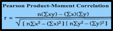
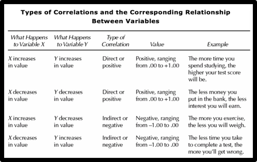 A perfect correlation of 1 or -1 indicates that the value of one variable can be determined exactly by knowing the value on the other variable. A scatterplot of this relationship Will be a straight line. 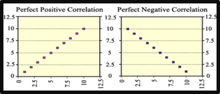 A correlation of 0 indicates no relationship between the two variables. Knowing the value of one of the variables provides no assistance in predicting the value of the second variable. A scatterplot will be a circle of points. 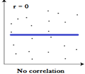 Assumptions There are a number of assumptions that we need to check before conducting the correlation analysis. They are as follows: 1. Level of Measurement The scale of measurement for the variables ( IVs & DV) should be interval or ratio (continuous). According to Pallant ( 2013), if our independent variable is dichotomous variable (with only two values: e.g. sex) and the level of measurement of our dependent variable is interval or ratio, we can use Pearson Correlation. 2. Independence of Observations The observations that make up your data must be independent of one another. 3. Normality Distribution fo our data should be normal. Normality of our variables can be checked using histograms, stem and leaf display, Box plot. WE can also check the value of Skewness and mean, median, and mode of our variable (Mean=Median=mode). 4. Linearity The relationship between the two variables should be linear. This assumption can be checked by generating a scatter plot. 5. Homoscedasticity —The variability in scores for variable X should be similar at all values of variable Y. This assumption can be checked by generating a scatter plot. A scatter plot should show a fairly even cigar shape along its length. 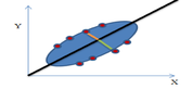 —Before performing a correlation analysis, we should generate a scatterplot. This enables us to check for violation of the assumptions of linearity and homoscedasticity. Also, inspection of the scatterplots gives us a better idea of the direction and the strength of the linear relationship between two variables. 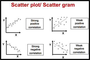 Components of Pearson product-moment correlationPearson correlation analysis consists of two parts : 1. Discriptive and 2. Inferential 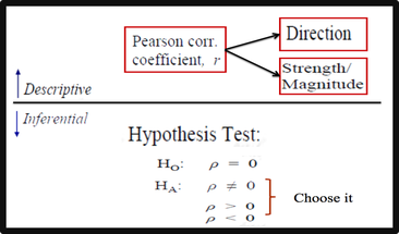 Descriptive: First, we should calculate Pearson Correlation Coefficient. Based on the value of the r, we can discribe the the direction and the strength of the linear relationship between two variables. we can use the following formula to calculate the correlation coefficient. 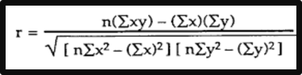 How to Interpret a Correlation Coefficient r we can use the following Rule of Thumb to interpret the r value. 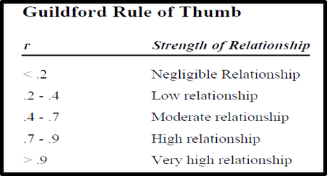 Inferential: Second, we test the hypotheis to find out whether there is a significant relationship between two variables. Steps in Hypothesis Testing using Excel 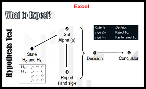 Coefficient of determination We can calculate coefficient of determination to determin how much variance our two variables share. In other words, it shows the amonunt of total variance in dependent variable that can be explained by independent variables. A coefficient of determination ( R square) can be calculated by multiplying r value by itself. To convert this to 'percentage of variance', just multiply by 100. For example, two variables that correlate r=.4 share only (.4 x .4 = .04 = 16) 16 per cent of their variance. Excel or Spss can calculate the R square or coefficient of determination for us. How to calculate correlation analysis using Excel and write up the findings for a report How to Make and Interpret a Scatter Plot in Excel Excel: Two Scatterplots and Two Trendlines
1 Comment
|
Categories
All
|
 RSS Feed
