 Simple Linear Regression is a modeling technique. It is based on correlation and can be used to explore the relationship between one continuous dependent variable and one continuous independent variable or predictor. In this way, we can find out whether an independent variable can make significant unique contribution to the prediction of the dependent variable. In addition, Simple Linear Regression can be used to explore the predictive ability of the model. Simple Linear Regression will provide us with information about the model as a whole and the relative contribution of the independent variable that make up the model. In other words, Simple Linear Regression tells us how much of the variance in our dependent variable can be explained by our independent variable. It also gives us an indication of the relative contribution of our independent variable. To put it in a nutshell, Simple Linear Regression is used
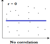
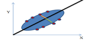
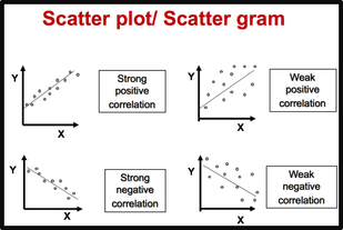
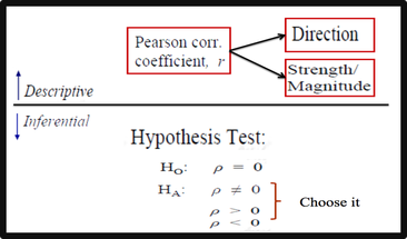
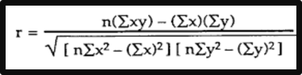
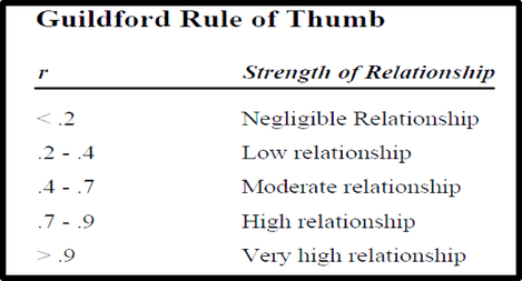
What we need: One continuous dependent variable and one continuous independent variable (we can also use dichotomous independent variables, e.g. males=l, females=2.) Assumptions: Before performing this analysis, we should check several assumptions such as Normality, linearity, homoscedasticity, independence of observations, and Outliers. Steps in Regression Analysis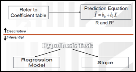 Simple Linear Regression consists of two parts: Descriptive & Inferential Descriptive: 1. The Correlation Coefficient (r): Based on r value, we describe the strength and direction of the linear relationship between two continuous variables 2. The Coefficient of Determination (R Square): Based on R square, we can say that how much of the total variance in the dependent variable is uniquely explained by an independent variable. 3. Prediction Equation or Regression Model: Regression Model involves statistics and parameters, namely: Intercept and slope of the regression line. 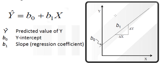 2. Inferential we should Test two objectives: 1. To explore predictive ability of the model (To determine whether the model really fits the data. 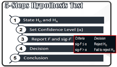 2. To determine the significance of the relationship between IV and DV ( To test whether an independent variable is making significant unique contribution to the prediction of the dependent variable.) 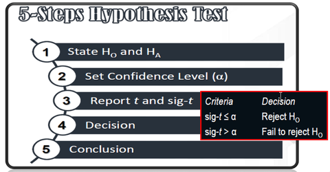 Linear Regression using Excel |
|||||||||


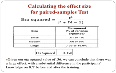 |
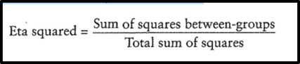
The guidelines (proposed by Cohen 1988, pp. 284–7) for interpreting this value are: .01=small effect, .06=moderate effect, .14=large effect. Given our eta squared value of .35 we can conclude that there was a large effect, with a substantial difference in knowledge of ICT scores obtained before and after the intervention.
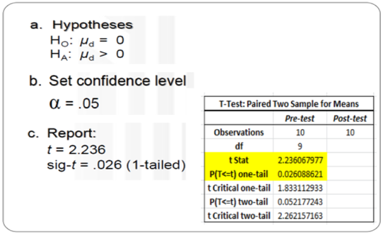
Presenting the results for paired-samples t-test
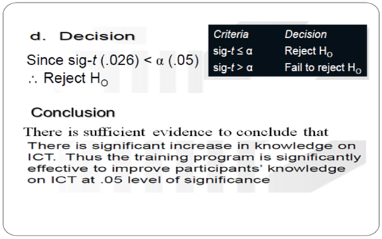
A paired-samples t-test was conducted to evaluate the impact of the training on participants’ knowledge of ICT scores. There was a statistically significant increase in participants’ knowledge of ICT scores from Pre test (Time 1) (M = 12.3, SD = 0.59) to post test (Time 2) (M = 12.8, SD = 0.69), t = 2.23, p <. 05 (one-tailed). The mean increase in Participants’ knowledge of ICT scores was 0.5 with a 95% confidence interval. The eta squared statistic (.35) indicated a large effect size.
Presenting the results for paired-samples t-test
A paired-samples t-test was conducted to evaluate the impact of the training on participants’ knowledge of ICT scores. There was a statistically significant increase in participants’ knowledge of ICT scores from Pre test (Time 1) (M = 12.3, SD = 0.59) to post test (Time 2) (M = 12.8, SD = 0.69), t = 2.23, p <. 05 (one-tailed). The mean increase in Participants’ knowledge of ICT scores was 0.5 with a 95% confidence interval. The eta squared statistic (.35) indicated a large effect size.
z test is used to test the difference between two means when the population standard deviations are known and the variables are normally or approximately normally distributed. In many situations, however, these conditions cannot be met—that is, the population standard deviations are not known. In these cases, a t test is used to test the difference between means.
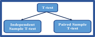
There are a number of different types of t-tests. The two that will be discussed here are:
• Independent-samples t-test, used when we want to compare the mean scores of two different groups of people or conditions; and
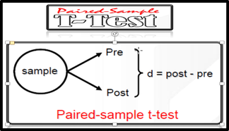
• Paired-samples t-test, used when we want to compare the mean scores for the same group of people on two different occasions, or when we have matched pairs.
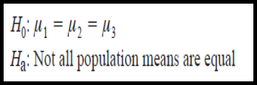
In both cases, we are comparing the values on some continuous variable for two groups or on two occasions. If we have more than two groups or conditions, we will need to use analysis of variance instead.
There are a number of different types of t-tests. The two that will be discussed here are:
• Independent-samples t-test, used when we want to compare the mean scores of two different groups of people or conditions; and
• Paired-samples t-test, used when we want to compare the mean scores for the same group of people on two different occasions, or when we have matched pairs.
In both cases, we are comparing the values on some continuous variable for two groups or on two occasions. If we have more than two groups or conditions, we will need to use analysis of variance instead.
Assumptions
For both of the t-tests that I discuss here, there are a number of assumptions that we will need to check before conducting these analyses.
Level of measurement
Each of the parametric approaches assumes that the dependent variable is measured at the interval or ratio level; that is, using a continuous scale rather than discrete categories. When we want to design our study, we should try to make use of continuous, rather than categorical for the dependent variable. This gives us a wider range of possible techniques to use when analyzing our data.
Random sampling
Data should be collected using a random sample from the population.
Independence of observations
The observations that make up our data must be independent of one another; that is, each observation must not be influenced by any other observation. Violation of this assumption, according to Stevens (1996, p. 238), is very serious. There are a number of research situations that may violate this assumption of independence. For example:
- We are interested in studying the performance of students working in pairs or small groups. The behaviour of each member of the group influences all other group members, thereby violating the assumption of independence.
- Studying the TV-watching habits and preferences of children drawn from the same family. The behaviour of one child in the family (e.g. watching Program A) is likely to influence all children in that family; therefore, the observations are not independent.
Normal distribution
For parametric techniques, it is assumed that the populations from which the samples are taken are normally distributed. In a lot of research scores on the dependent variable are not normally distributed. Fortunately, most of the techniques are reasonably 'robust' or tolerant of violations of this assumption. With large enough sample sizes (e.g. 30+), the violation of this assumption should not cause any major problems. Normality of our variables can be checked using histograms, stem and leaf display, Box plot. WE can also check the value of Skewness and mean, median, and mode of our variable (Mean=Median=mode).
Homogeneity of variance
Samples that are obtained from populations should have equal variances. This means that the variability of scores for each of the groups is similar.
Independent Sample T-test
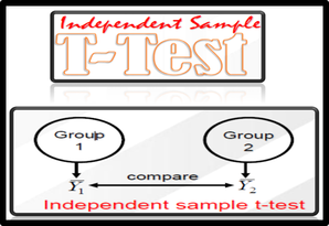
Purpose of Independent sample t-test
—To compare differences between two (2) independent group means
Requirements
►DV–Interval or ratio
►IV–Nominal or ordinal (k=2)
►IV–Nominal or ordinal (k=2)
| Example of research question: Is there a significant difference in the mean self esteem scores for males and females? What we need: Two variables:
How to test the hypothesis for the independent sample t-test 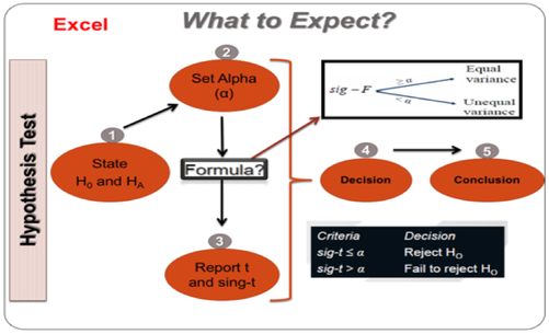 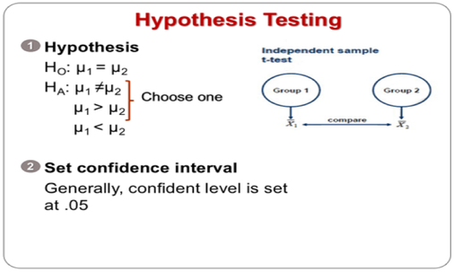 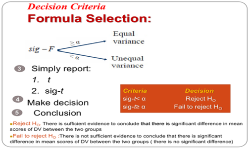 |
Interpretation of output from independent-samples t-test
Step 1: Checking the information about the groups
Excel gives us the mean and standard deviation for each of our groups (in this case, Support/ Admin). It also gives us the number of people in each group (N). We should always check these values first. Are the N values for support and Admin correct? Or are there a lot of missing data? If so, we should find out why. Perhaps we have entered the wrong code for Support and females (0 and 1, rather than 1 and 2). We should check our codebook.
Step 2: Checking assumptions
The independent sample t-test assumes the variances of the two groups we are measuring are equal in the population. If our variances are unequal, this can affect the Type I error rate. We should run the F-test two sample for variances in Excel to check the equality of variances. This tests whether the variance (variation) of scores for the two groups (Support and Admin) is the same. If Sig-F is grater than the significance value (Sig-F ≥ œ), the T-test: two sample assuming equal variances can be used. If Sig-F is less than the level of significance (Sig-F≤ œ), the test for equality of variances is statistically significant. It indicates that the group variances are unequal in the population. We can correct this violation by using the T-test: two sample assuming unequal variances.
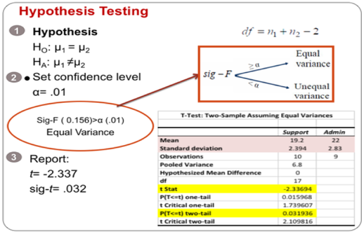
In this case, Sig-F is larger than alpha value so we can use the T-test: two sample assuming equal variances.
We should also check other assumptions such as level of measurement, random sampling, independence of observations, and normality of our data.
Step 3: Assessing differences between the groups
To find out whether there is a significant difference between our two groups, we should compare P-value ( Sign-t) with the level of significance.
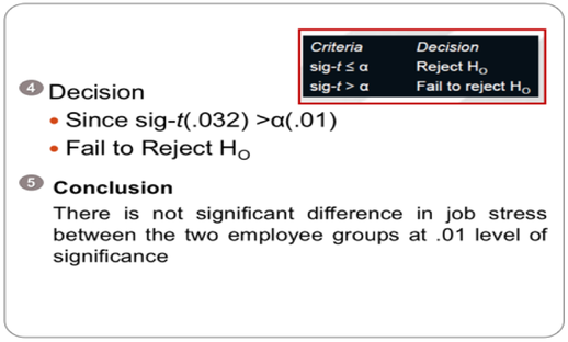
In the example presented in the output above, the P value (Sig. t- 2-tailed) is .03. As this value is above the required cut-off of .01, we conclude that there is not a statistically significant difference in the mean Job stress scores for Support and Admin group.
Calculating the effect size for independent-samples t-test
One way that we can assess the importance of our finding is to calculate the effect size. Effect size statistics provide an indication of the magnitude of the differences between our groups (not just whether the difference could have occurred by chance).
There are a number of different effect size statistics, the most commonly used are eta squared and Cohen’s d. Eta squared can range from 0 to 1 and represents the proportion of variance in the dependent variable that is explained by the independent (group) variable.
We can use a formula to calculate the eta squared.
Step 1: Checking the information about the groups
Excel gives us the mean and standard deviation for each of our groups (in this case, Support/ Admin). It also gives us the number of people in each group (N). We should always check these values first. Are the N values for support and Admin correct? Or are there a lot of missing data? If so, we should find out why. Perhaps we have entered the wrong code for Support and females (0 and 1, rather than 1 and 2). We should check our codebook.
Step 2: Checking assumptions
The independent sample t-test assumes the variances of the two groups we are measuring are equal in the population. If our variances are unequal, this can affect the Type I error rate. We should run the F-test two sample for variances in Excel to check the equality of variances. This tests whether the variance (variation) of scores for the two groups (Support and Admin) is the same. If Sig-F is grater than the significance value (Sig-F ≥ œ), the T-test: two sample assuming equal variances can be used. If Sig-F is less than the level of significance (Sig-F≤ œ), the test for equality of variances is statistically significant. It indicates that the group variances are unequal in the population. We can correct this violation by using the T-test: two sample assuming unequal variances.
In this case, Sig-F is larger than alpha value so we can use the T-test: two sample assuming equal variances.
We should also check other assumptions such as level of measurement, random sampling, independence of observations, and normality of our data.
Step 3: Assessing differences between the groups
To find out whether there is a significant difference between our two groups, we should compare P-value ( Sign-t) with the level of significance.
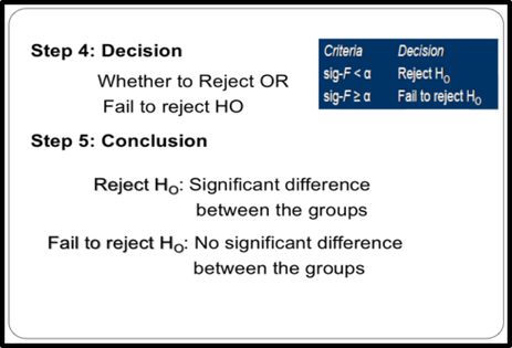
- If the P value (Sig-t) is equal or less than .05 or 0.01 , we reject the null hypothesis. So, we can conclude that there is a significant difference in the mean scores on our dependent variable for the two groups.
- If the P value (Sig-t) is above .05 or 0.01 , we fail to reject the null hypothesis. So, we can conclude that there is not a significant difference between the two groups.
In the example presented in the output above, the P value (Sig. t- 2-tailed) is .03. As this value is above the required cut-off of .01, we conclude that there is not a statistically significant difference in the mean Job stress scores for Support and Admin group.
Calculating the effect size for independent-samples t-test
One way that we can assess the importance of our finding is to calculate the effect size. Effect size statistics provide an indication of the magnitude of the differences between our groups (not just whether the difference could have occurred by chance).
There are a number of different effect size statistics, the most commonly used are eta squared and Cohen’s d. Eta squared can range from 0 to 1 and represents the proportion of variance in the dependent variable that is explained by the independent (group) variable.
We can use a formula to calculate the eta squared.
Presenting the results for independent-samples t-test
The results of the analysis can be presented as follows:
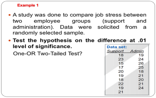
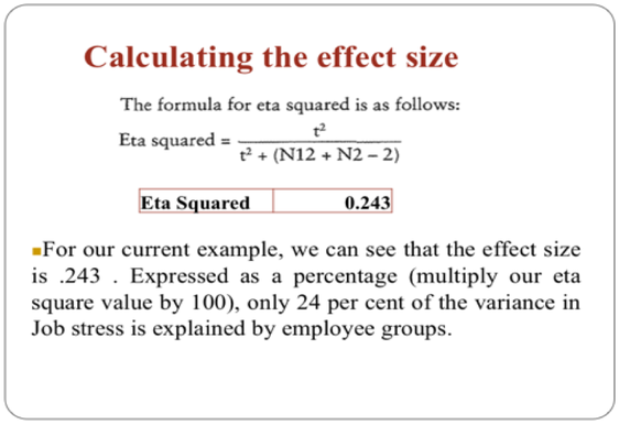
An independent-samples t-test was conducted to compare the job stress scores for Support and Admin groups. There was no significant difference in the mean Job stress scores for Support (M = 19.2, SD = 2.39) and Admin groups (M = 22, SD = 2.83) at 0.01 (t = -2.336, p = .03, two-tailed). Eta squared was 0.243 ( 24% of of variance in the Job stress is explained by the employee groups). The magnitude of the differences in the means (mean difference = 2.8,) was 1.07 .
The results of the analysis can be presented as follows:
An independent-samples t-test was conducted to compare the job stress scores for Support and Admin groups. There was no significant difference in the mean Job stress scores for Support (M = 19.2, SD = 2.39) and Admin groups (M = 22, SD = 2.83) at 0.01 (t = -2.336, p = .03, two-tailed). Eta squared was 0.243 ( 24% of of variance in the Job stress is explained by the employee groups). The magnitude of the differences in the means (mean difference = 2.8,) was 1.07 .

The difference between qualitative & quantitative Research Method
Two main types of research method are Qualitative and Quantitative research method.
These two types of research method are different fundamentally.
Qualitative Research is primarily exploratory research. It is used to gain an in-depth understanding of underlying reasons, opinions, and motivations. It provides insights into the problem or helps to develop ideas or hypotheses for potential quantitative research. Qualitative Research is also used to uncover trends in thought and opinions, and dive deeper into the problem. Qualitative data collection methods vary using unstructured or semi-structured techniques. Some common methods include focus groups (group discussions), individual interviews, and participation/observations. The sample size is typically small, and respondents are selected to fulfill a given quota.
Quantitative Research is used to quantify the problem by way of generating numerical data or data that can be transformed into useable statistics. It is used to quantify attitudes, opinions, behaviors, and other defined variables – and generalize results from a larger sample population. Quantitative Research uses measurable data to formulate facts and uncover patterns in research. Quantitative data collection methods are much more structured than Qualitative data collection methods. Quantitative data collection methods include various forms of surveys – online surveys, paper surveys, mobile surveys and kiosk surveys, face-to-face interviews, telephone interviews, longitudinal studies, website interceptors, online polls, and systematic observations.
The difference between descriptive and inferential statistics
Descriptive statistics can be used to describe and summarize the characteristics of a data set. On the other hand, Inferential statistics can be used to test a hypothesis or assess whether our data is generalizable to the broader population.
In the case that the population size of our study is large, we should select the sample and data will be collected from the sample. Results obtained from the sample can be generalized to an entire population of interest through the testing of hypothesis which is a decision-making process for evaluating claims about a population. In fact, setting up and testing hypotheses is an essential part of statistical inference.
There are two types of statistical hypotheses for each situation:
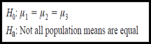
1. The null hypothesis
2. The alternative hypothesis.
These two types of research method are different fundamentally.
Qualitative Research is primarily exploratory research. It is used to gain an in-depth understanding of underlying reasons, opinions, and motivations. It provides insights into the problem or helps to develop ideas or hypotheses for potential quantitative research. Qualitative Research is also used to uncover trends in thought and opinions, and dive deeper into the problem. Qualitative data collection methods vary using unstructured or semi-structured techniques. Some common methods include focus groups (group discussions), individual interviews, and participation/observations. The sample size is typically small, and respondents are selected to fulfill a given quota.
Quantitative Research is used to quantify the problem by way of generating numerical data or data that can be transformed into useable statistics. It is used to quantify attitudes, opinions, behaviors, and other defined variables – and generalize results from a larger sample population. Quantitative Research uses measurable data to formulate facts and uncover patterns in research. Quantitative data collection methods are much more structured than Qualitative data collection methods. Quantitative data collection methods include various forms of surveys – online surveys, paper surveys, mobile surveys and kiosk surveys, face-to-face interviews, telephone interviews, longitudinal studies, website interceptors, online polls, and systematic observations.
The difference between descriptive and inferential statistics
Descriptive statistics can be used to describe and summarize the characteristics of a data set. On the other hand, Inferential statistics can be used to test a hypothesis or assess whether our data is generalizable to the broader population.
In the case that the population size of our study is large, we should select the sample and data will be collected from the sample. Results obtained from the sample can be generalized to an entire population of interest through the testing of hypothesis which is a decision-making process for evaluating claims about a population. In fact, setting up and testing hypotheses is an essential part of statistical inference.
- Hypothesis is a claim or idea about a group or population.
- Hypothesis refers to an educated guess or assumption that can be tested.
- Hypothesis is formulated based on previous studies.
- A good hypothesis should be simple, concise and testable.
There are two types of statistical hypotheses for each situation:
1. The null hypothesis
2. The alternative hypothesis.
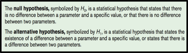
The null hypothesis is opposite of alternative hypothesis. If we can prove that the null hypothesis is false , then we can conclude that the research or alternative hypothesis is true.
Example:
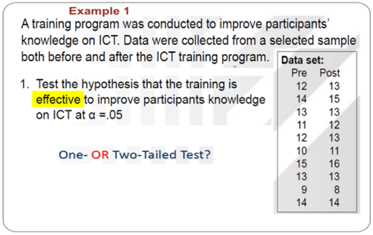
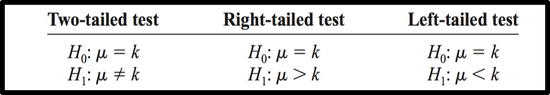
One-Tailed Test & Two-Tailed Test
There are two forms of research hypothesis.
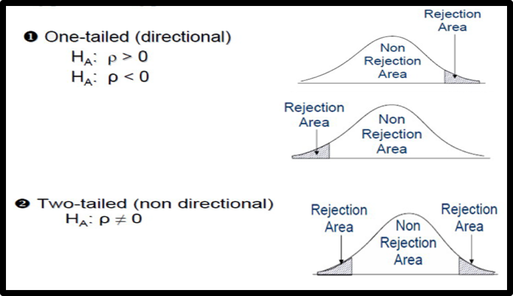
The critical or rejection region can be one side of the distribution or both sides of the distribution depending on the nature of the research hypothesis.
Directional research hypothesis or one tail test has one critical region. On the contrary, the Non-directional research hypothesis or two tail test has two rejection regions on both sides of the distribution.
How to determine if it is a one tailed or two tailed test?
Write the null and alternative hypothesis for the following situations.
Situation A
A medical researcher is interested in finding out whether a new medication will have any undesirable side effects. He knows that the mean pulse rate for the population under study is 82 beats per minute. Hence, he tries to find whether the pulse rate will increase, decrease, or remain unchanged after a patient takes the medication?
The hypotheses for this situation are
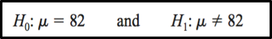
The null hypothesis specifies that the mean will remain unchanged, and the alternative hypothesis states that it will be different. This test is called a two-tailed test , since the possible side effects of the medicine could be to raise or lower the pulse rate.
Situation B
A chemist invents an additive to increase the life of an automobile battery. If the mean lifetime of the automobile battery without the additive is 36 months, then her hypotheses are :
Situation B
A chemist invents an additive to increase the life of an automobile battery. If the mean lifetime of the automobile battery without the additive is 36 months, then her hypotheses are :
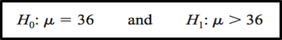
In this situation, the chemist is interested only in increasing the lifetime of the batteries, so her alternative hypothesis is that the mean is greater than 36 months. The null hypothesis is that the mean is equal to 36 months. This test is called right-tailed, since the interest is in an increase only.
Situation C
A contractor wishes to lower heating bills by using a special type of insulation in houses. If the average of the monthly heating bills is $78, her hypotheses about heating costs with the use of insulation are
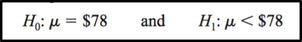
To state hypotheses correctly, researchers must translate the conjecture or claim from words into mathematical symbols. The basic symbols used are as follows:
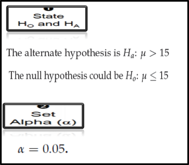
Level of Significance ( alpha value)
The conclusion of the hypothesis testing must be attached to the level of confidence at which we reject the null hypothesis. Level of confidence is expressed as 90%, 95%, 99% and so on. By convention, the .05 level of significance has been considered an acceptable significant level in social science studies.
0.05 level of significance means that we are 95% confident that we have made the right decision and only 5% of incurring error. The smaller the significance level indicates, the more stringent the hypothesis testing.
Critical Region
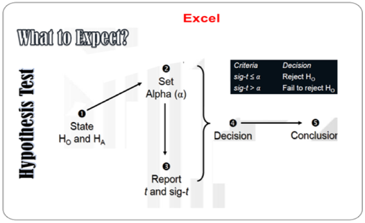
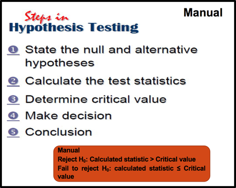
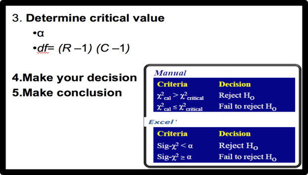
Knowledge of sampling distribution enables us to decide whether to reject or fail to reject the null hypothesis. The decision is based on two criteria: the critical value of the test statistics and the significance level.
The critical value is obtained from the test statistic table (e.g., Z, t, f table) corresponding to the level of significance and degrees of freedom.
If the value of the test statistics is greater than the critical value, we reject the null hypothesis. In other words, we reject the null hypothesis if the value of the test statistic falls beyond the critical value and within the critical region.
On the other hand, if the value of the test statistics is smaller than the critical value, we fail to reject the null hypothesis.
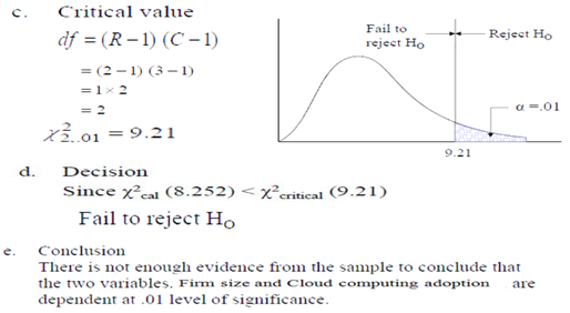
- Reject H0: Calculated statistic > Critical value
- Fail to reject H0: calculated statistic ≤ Critical value
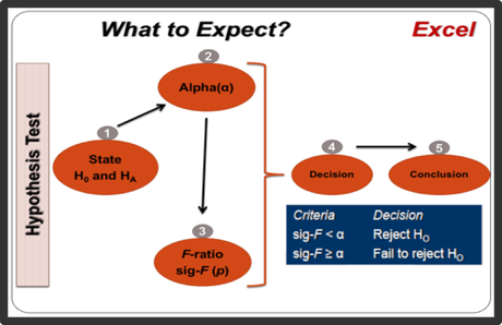
Also, if the P value (Sig-value) is smaller than the level of significance, we reject the null hypothesis. On the contrary, if the P value (Sig-value) is greater than the level of significance, we fail to reject the null hypothesis.
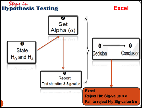
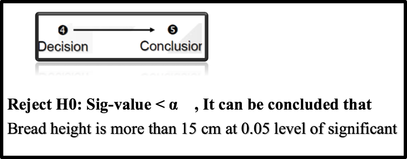
- Reject H0: Sig-value < α
- Fail to reject H0: Sig-value ≥ α
Type 1 Error, Type 2 Error & Power
In every study, there is a chance for error. In other words, there is always the possibility of reaching the wrong conclusion. There are two different errors that we can make, Type 1 error and Type 2 error.
Type 1 Error: We may reject the null hypothesis when it is, in fact, true. This occurs when we think there is a difference between our groups, but there really isn’t. We can minimise this possibility by selecting an appropriate alpha level .
Type 2 Error: Type 2 error occurs when we fail to reject a null hypothesis when it is, in fact, false (i.e. believing that the groups do not differ, when in fact they do).
Unfortunately, these two errors are inversely related. As we try to control for a Type 1 error, we actually increase the likelihood that we will commit a Type 2 error.
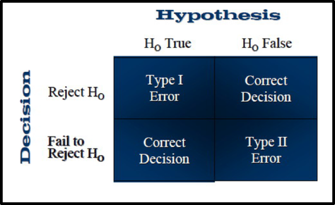
Ideally, we would like to make the correct decision.
This is called the power of a test. There are several factors that can influence the power of a test in a given situation:
- sample size
- effect size (the strength of the difference between groups, or the influence of the
- independent variable)
- alpha level set by the researcher (e.g. .05/.01).
The power of a test is very dependent on the size of the sample used in the study. According to Stevens (1996), when the sample size is large (e.g. 100 or more participants) power is not an issue . However, when the sample size is small, the result of our test may be non- significant. This result may be due to insufficient power. Stevens (1996) suggests that when small group sizes are involved it may be necessary to adjust the alpha level to compensate (e.g. set a cut-off of .10 or .15, rather than the traditional .05 level).
Cohen ( 1988) created "Power Tables for Effect Size d" that will tell us how large our sample size need to achieve sufficient power, given the effect size we wish to detect. There are also a growing number of software programs that can do these calculations for us (e.g. G*Power ; and UnifyPow (SAS)).
The standard power is 80% . It means the probability of making a correct decision is 80% and 20 % of incurring error. If we obtain a non-significant result and are using quite a small sample size, we should check the power value. If the power of the test is less than 80%, we need to interpret the reason for our non-significant result carefully. This may suggest insufficient power of the test, rather than no real difference between our groups.
The power analysis gives an indication of how much confidence we should have in the results when we fail to reject the null hypothesis. The higher the power, the more confident we can have that our result is correct ( there is no real difference between the groups).
Types of Power Analyses
A priori
* before the study is conducted
*helps in the design of study
Post hoc
*done after the study is conducted
*helps to understand observed results
Compromise
*done when sample size is restricted
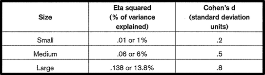
Effect Size
One way that we can assess the importance of your finding is to calculate the 'effect size' (also known as 'strength of association'). This is a set of statistics that indicates the relative magnitude of the differences between means, or the amount of the total variance in the dependent variable that is predictable from knowledge of the levels of the independent variable (Tabachnick & Fidell 2013).
There are a number of different effect size statistics. The most commonly used to compare groups are partial eta squared and Cohen's d.
Partial eta squared effect size statistics indicate the proportion of variance of the dependent variable that is explained by the independent variable. Values can range from 0 to 1. Cohen's d, on the other hand, presents difference between groups in terms of standard deviation units.
(Effect size calculators is a useful website that provides a quick and easy way to calculate effect size statistics )
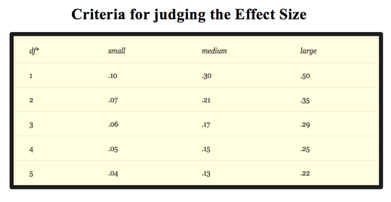
Cohen ( 1988) proposed a guideline that can be used to interpret the strength of the different effect size statistics.
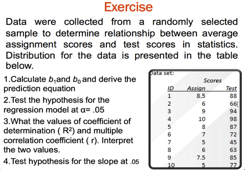
Exercise
1. Describe the importance of descriptive and inferential statistics in research?
2. Which of the following is the highest type 1 error ? Explain why?
a. α= .100
b. α= .01
c. α=.001
d. α=.0001
3. A researcher tested a hypothesis at the 0.05 significance level. Explain the meaning of this statement.
4. Explain factors that should be considered before choosing a specific statistical procedure.
5. State the null and alternative hypotheses for each conjecture.
a. A researcher thinks that if expectant mothers use vitamin pills, the birth weight of the babies will increase. The average birth weight of the population is 8.6 pounds.
b. An engineer hypothesizes that the mean number of defects can be decreased in a manufacturing process of compact disks by using robots instead of humans for certain tasks. The mean number of defective disks per 1000 is 18.
c. A psychologist feels that playing soft music during a test will change the results of the test. The psychologist is not sure whether the grades will be higher or lower. In the past, the mean of the scores was 73.
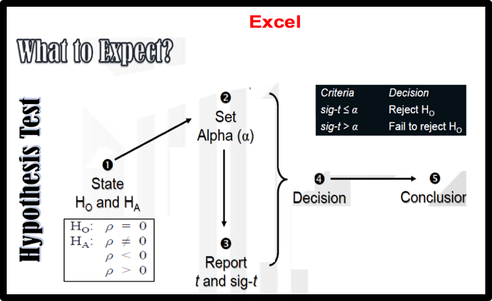
Steps in Hypothesis Testing
Example:
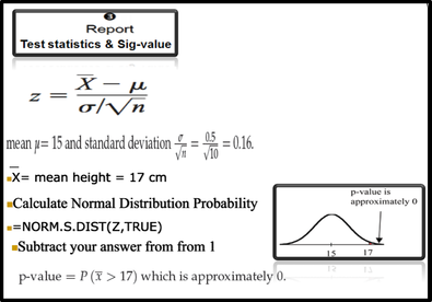
Suppose a baker claims that his bread height is more than 15 cm, on the average. Several of his customers do not believe him. To persuade his customers that he is right, the baker decides to do a hypothesis test. He bakes 10 loaves of bread. The mean height of the sample loaves is 17 cm. The baker knows from baking hundreds of loaves of bread that the standard deviation for the height is 0.5 cm. and the distribution of heights is normal.
(Since the problem is about a mean height, this is a test of a single population mean).
what is the difference between parametric and non-parametric techniques? Why is the distinction important?
Go to Socrative.com and click Student Login, Room Name. JOIN
https://b.socrative.com/login/student/
Room: AFSHARI2233
Go to Socrative.com and click Student Login, Room Name. JOIN
https://b.socrative.com/login/student/
Room: AFSHARI2233

Parametric & Non-Parametric Tests
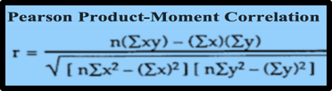
Parametric techniques like T-tests, Analysis of Variance, Pearson Product Moment Correlation, Regression are more powerful than non-parametric tests (e.g., Chi-square tests). If you have the right sort of data, it is always better to use a parametric technique because the results of these statistical techniques are more reliable. However, you should use non-parametric statistics in some situations. Non-parametric techniques are ideal for use when you have qualitative data (Nominal or Ordinal data) and small sample sizes. You can also use non-parametric techniques if the distribution of your data is not normal.
Parametric & Non-Parametric Tests
Parametric techniques like T-tests, Analysis of Variance, Pearson Product Moment Correlation, Regression are more powerful than non-parametric tests (e.g., Chi-square tests). If you have the right sort of data, it is always better to use a parametric technique because the results of these statistical techniques are more reliable. However, you should use non-parametric statistics in some situations. Non-parametric techniques are ideal for use when you have qualitative data (Nominal or Ordinal data) and small sample sizes. You can also use non-parametric techniques if the distribution of your data is not normal.

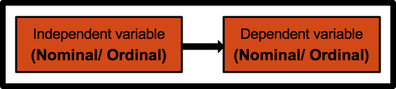
Chi-square test for independence is one of the most popular and versatile non-parametric tests. It is used to explore the association between two categorical variables. Each of these variables can have two or more categories.
Chi-square test for independence is one of the most popular and versatile non-parametric tests. It is used to explore the association between two categorical variables. Each of these variables can have two or more categories.
This test also compares the observed frequencies with the expected frequencies.
For example, we want to explore the association between Gender ( Male / Female) and Smoking Behaviour ( Smoker/Non-Smoker).
Independent and dependent variables are Gender and Smoking Behaviour respectively.
Both variables are categorical variables with two categories.
IV: Gender ( Male/ Female)
DV: Smoking Behaviour ( Smoker / Non Smoker)
Example of research question: There are a variety of ways questions can be phrased:
- Is there an association between gender and smoking behavior?
- Are males more likely to be smokers than females?
- Is the proportion of males that smoke the same as the proportion of females?
Several assumptions should be checked before conducting this analysis. Additional assumption that should be checked is the " Minimum Expected Cell Frequency".
Based on this assumption, the lowest expected frequency in any cell should be 5 or more. Some authors suggest less stringent criteria: at least 80 per cent of cells should have expected frequencies of 5 or more. If we have a 1 by 2 or a 2 by 2 table, it is recommended that the expected frequency be at least 10. If we have a 2 by 2 table that violates this assumption, we should consider using Fisher's Exact Probability Test instead
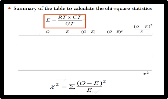
Steps to Solve a Chi-Square Test problem
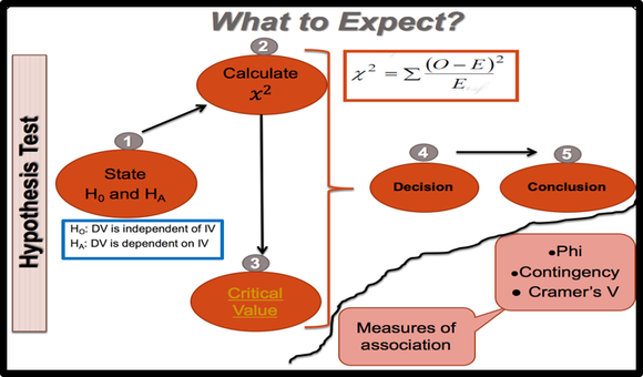
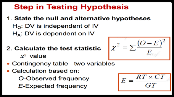
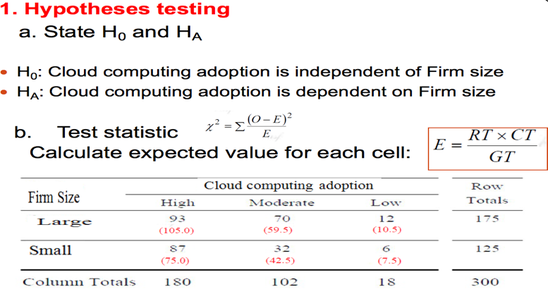
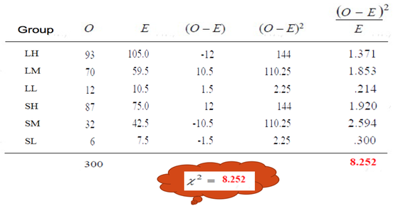
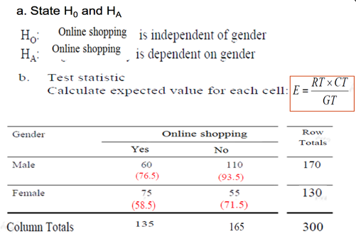
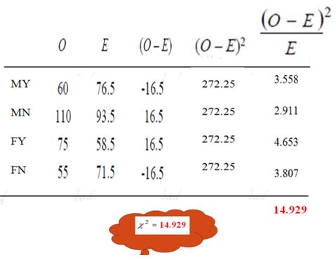
We should generate the Contingency table to calculate the Chi-Square statistics. We need two values, Observed frequency ( O) and Expected frequency ( E). Collected data are observed frequency and expected frequency can be calculated by the above formula.
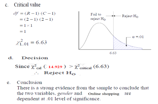
 Then, we should find the criticla value. The chi-square critical value can be any number between zero and plus infinity. We can use Chi-Square table to find the critical chi-square value. This value is based on the Level of significance and Degree of Freedom. (Excel and SPSS can calculate the critical chi-square for us.) For making decision, we can compare the critical chi-square with chi-square statistics OR we can compare P-value with Level of significance. (see the following criteria) |
Effect Size
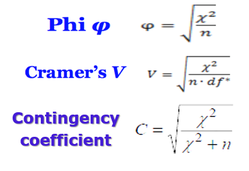
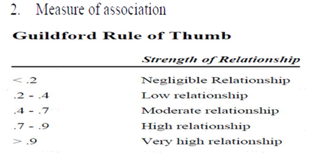
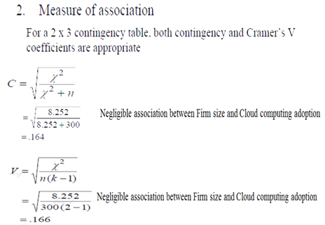
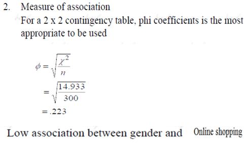
By testing hypothesis, we can show that our result is statistically is significant. But if we want to show that our result is theoretically and practically significant, we should find the effect size. There are a number of effect size statistics (such as Phi coefficient, Cramer's V, and Contingency coefficient) that can be used to determine the strength and magnitude of the association between two variables.
For 2 by 2 tables, the most commonly used one is the phi coefficient, which is a correlation coefficient and can range from 0-1, with higher values indicating a strong association between the two variables.
For tables larger than 2 by 2, the value to report is Cramer's V or Contingency coefficient.
Learn how to perform the chi-square test of independence with the following examples. ( Please watch the videos)
Crosstabulation with pivot table and chi-square test using Excel
| pearson_correlation_simple_linear_regression_chi-square.pdf |
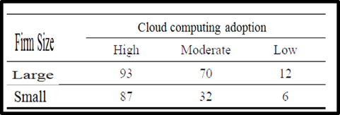
Example 1:
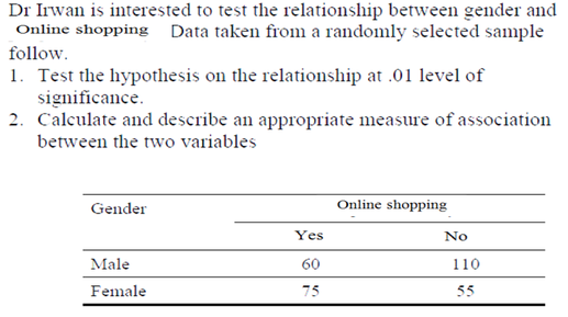
—A study was conducted to test the association between Firm size and cloud computing adoption. Data collected from a randomly selected sample follow.
—1. Test the hypothesis on the association between the
two variables at .01 level of significance.
—2. Calculate and describe an appropriate measure of
association between the two variables.
—1. Test the hypothesis on the association between the
two variables at .01 level of significance.
—2. Calculate and describe an appropriate measure of
association between the two variables.
Example 2
Categories
All
A. Hypothesis Testing : (Qualitative & Quantitative Research; One-tailed Test & Two-Tailed Test; Level Of Significance; Critical Region; Type 1 & 2 Error ; Power ; Effect Size; Steps In Hypothesis Testing)
A. Parametric & Non-Parametric Tests
B. Chi-square Test For Independence
C. Assumptions Of T-test & Independent Sample T-test
D. Paired-Sample T-test
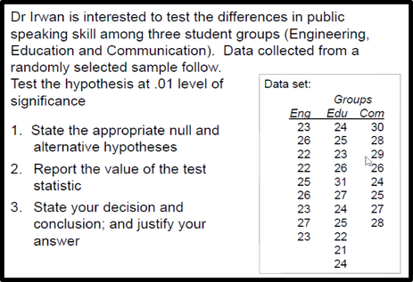
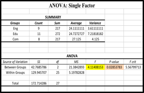
E. One-way ANOVA
F. Pearson Correlation
G.Simple Linear Regression
 RSS Feed
