Outliers
 Step 5: Identify Inter-Quartile Range IQR= Q3-Q2 IQR=17.5 - 8 = 9.5  .50% of all the numbers are between Q1 and Q3 Step 6: Multiply the IQR by 1.5 to determine outliers in a data set 9.5* 1.5= 14.25 An outlier is any number that is 14.25 less than Q1 or 14.25 more than Q3
 How to Find Outliers with Excel
0 Comments
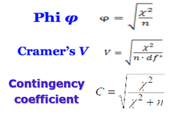
What is Percentile?
In general,
To find the percentile rank of a score, x, out of a set of n scores, where x is included: 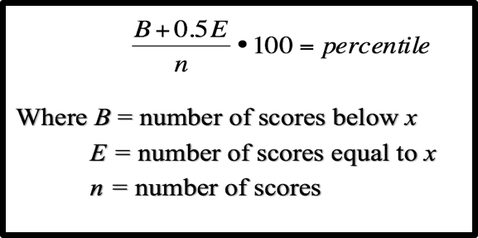 Example 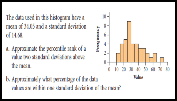 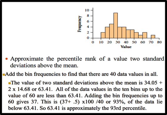 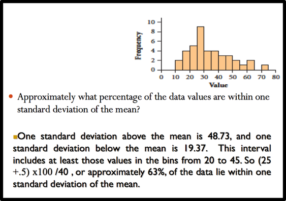 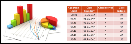 Organize data using a frequency distributionThe basic function of statistics is to organize and summarize data. Data collected in any research project are in raw and unorganized form. Not much meaning can be conveyed by raw data, unless the data are arranged or grouped in a certain manner to give more insight into the data. For example, I want to conduct a study to identify the level of customer loyalty in my company. In other words, I want to find out how many customers love my company and they will never choose another company. In this way, I can learn more about my customers. For collecting data, I can create an online questionnaire and distrubute randomly among my customers. After collecting data, I will have a big mass of data that is meaningless. To describe customer loyalty , draw conclusions, or make inferences about customer loyalty, I must organize the data in some meaningful way. The most convenient method of organizing data is to construct a frequency distribution. According to Bluman ( 2013), a frequency distribution is the organization of raw data in table form, using classes and frequencies. The reasons for constructing a frequency distribution are as follows:
Two types of frequency distributions that are most often used are the categorical frequency distribution and the grouped frequency distribution.
Grouped frequency distribution Suppose we want to identify the age of 50 students in the Statistics class. We first would have to get the data on the ages of the students. When the data are in original form, they are called raw data and are listed next. 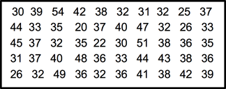 After collecting data, we will have a big mass of data that are raw and unorganized form. For organizing data, we should follow the following steps Steps in Organizing Data
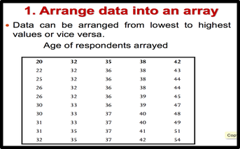
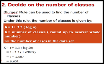
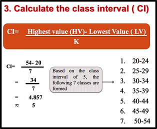
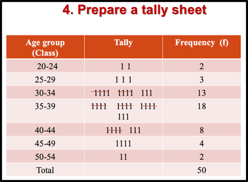
1: Arrange data into an array. The first step in organizing the data is to arrange them in an array so that we can observe the data in a more meaningful and systematic manner. Notice that data can be arranged from lowest to highest values (ascending order) or from highest to lowest values (descending order). 2: Decide on the number of classes (k) Before constructing the classes, we need to decide on the number of classes. As a general guide the recommended class number should be between 5 and 20. However, it’s just a guide. The class number can be less than 5 or more than 20. Another guideline that can be used in deciding the number of classes is to use the Sturges’ Rule. 3: Calculate the class interval (CI) 4. Prepare a tally sheet A tally sheet is important to calculate the frequency of cases in each of the seven classes.
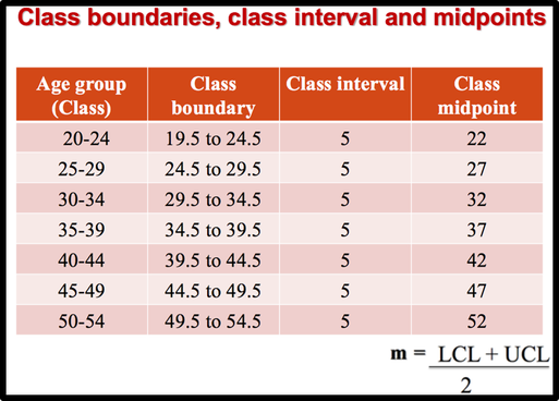 In the above distribution, the values 20 and 24 of the first class are called class limits. The lower class limit is 20; it represents the smallest data value that can be included in the class. The upper class limit is 24; it represents the largest data value that can be included in the first class. Class boundaries: These numbers are used to separate the classes so that there are no gaps in the frequency distribution. The gaps are due to the limits; for example, there is a gap between 24 and 25. we can find the boundaries by subtracting 0.5 from 20 (the lower class limit) and adding 0.5 to 24 (the upper class limit). Keep in mind that classes must be mutually exclusive. Mutually exclusive classes have nonoverlapping class limits so that data cannot be placed into two classes. To find class boundaries:
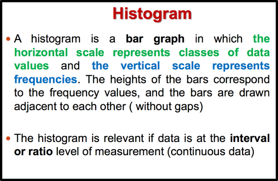
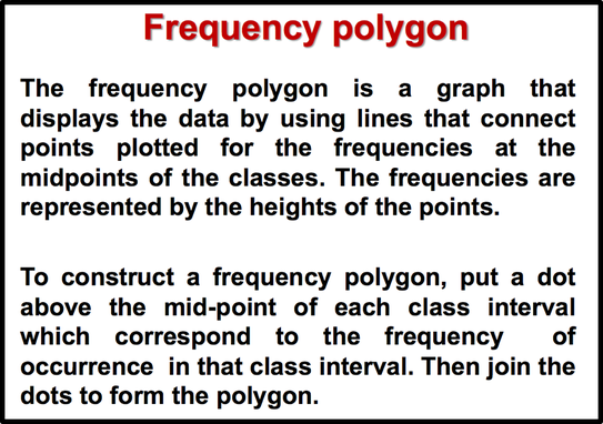
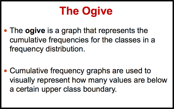
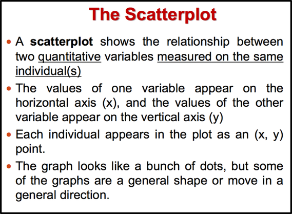
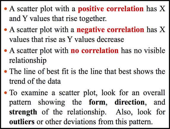
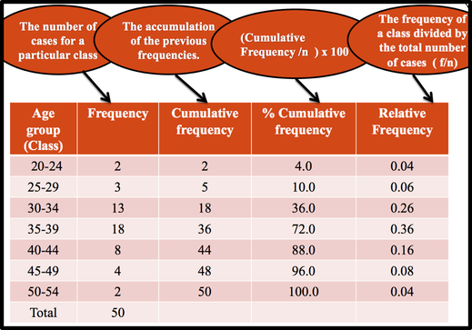 A cumulative frequency distribution ( CF) is a distribution that shows the number of data values less than or equal to a specific value (usually an upper boundary). It is obtained by adding the frequency for that class and all previous classes. Naturally, a shorter way to do this would be to just add the cumulative frequency of the class below to the frequency of the given class. For example, we can say that 18 ( 36%) students are less than or equal to 34.5 years in the third class. Alternatively, 32 (64%) of students are 34.5 years or more. Relative Frequency shows the proportion of data values that fall into a given class. In some situation, Relative frequency is more important than the actual number of data values that fall into that class. For example, if we want to compare the age distribution of students in statistics class with the age distribution of students in accounting class, you would use relative frequency distributions. The reason is that since the population of these two classes are different. To convert a frequency into a proportion or relative frequency, we should divide the frequency for each class by the total of the frequencies. The sum of the relative frequencies will always be 1. Frequency Distribution Table in Excel Elementary Statistics Lab Using Excel: Find Midpoints, Frequency, Rel Frequency, Cumulative Frequency, Cumulative Relative Frequency 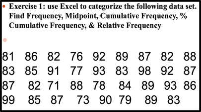 Use an Excel Pivot Table to Group Data by Age Bracket Categorical Frequency Distributions --The categorical frequency distribution is used for data that can be placed in specific categories, such as nominal- or ordinal-level data. For example, data such as political affiliation, religious affiliation, or major field of study would use categorical frequency distributions. Statistical GraphsAfter you have organized the data into a frequency distribution, you can present them in graphical form. The purpose of graphs in statistics is to convey the data to the viewers in pictorial form. It is easier for most people to comprehend the meaning of data presented graphically than data presented numerically in tables or frequency distributions. This is especially true if the users have little or no statistical knowledge. Statistical graphs can be used to describe the data set or to analyze it. Graphs are also useful in getting the audience’s attention in a publication or a speaking presentation. They can be used to discuss an issue, reinforce a critical point, or summarize a data set. They can also be used to discover a trend or pattern in a situation over a period of time. There are many different types of graphs but each one has a specific purpose. I divided statistical graphs into two categories . 1. Statistical graphs that can be used for quantitative data :
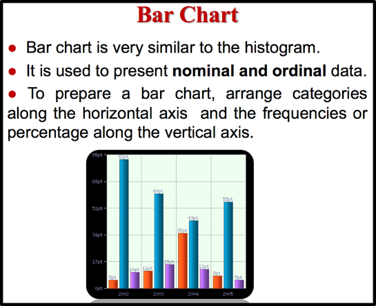
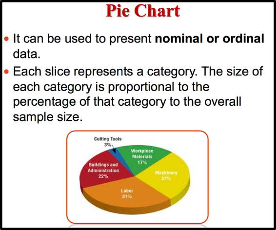
2. Statistical graphs that can be used for qualitative data :
|
| |
***Statistical graphs that can be used for qualitative data***
 |
Summary
- When data are collected, the values are called raw data. Since very little knowledge can be obtained from raw data, they must be organized in some meaningful way. A frequency distribution using classes is the common method that is used.
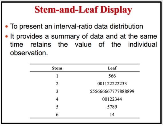
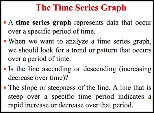
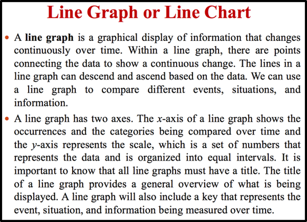
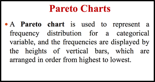
- Once a frequency distribution is constructed, graphs can be drawn to give a visual representation of the data. The most commonly used graphs in statistics are the histogram, frequency polygon, ogive, stem and leaf plot, bar graph, Pareto chart, time series graph, and pie graph .
Symmetric and Asymmetric Distributions
Frequency distribution can have two different shapes: Symmetric or asymmetric distribution. Asymmetric distribution can be positively skewed and negatively skewed distribution.
Symmetric Distribution
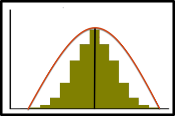
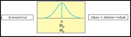
When the data values are evenly distributed about the mean, a distribution is said to be a symmetric distribution. A symmetry distribution ( normal distribution) resembles a bell-shape where the left portion of the distribution is equal to the right portion of the distribution. In addition, when the distribution is symmetric/unimodal , the mean, median, and mode are the same and are at the center of the distribution.
Symmetric Distribution
When the data values are evenly distributed about the mean, a distribution is said to be a symmetric distribution. A symmetry distribution ( normal distribution) resembles a bell-shape where the left portion of the distribution is equal to the right portion of the distribution. In addition, when the distribution is symmetric/unimodal , the mean, median, and mode are the same and are at the center of the distribution.
Asymmetric Distribution
—When there is higher density of observations on either side of the distribution, then the distribution is said to be an asymmetric distribution or Skewed (the majority of data values fall to the left or right of the mean).
Skewness
--Skewness is the degree of departure from symmetry of a distribution.
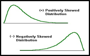
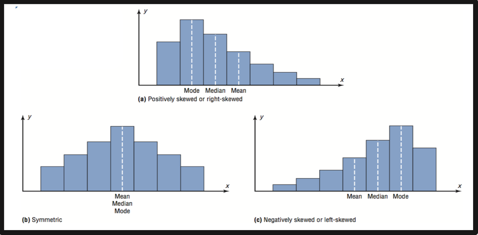
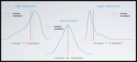
In a positively skewed or right-skewed distribution, the majority of data values fall to the left of the mean and cluster at the lower end of the distribution. The tail of the distribution goes to the larger values . In other words, the tail is to the right.
In a positively skewed distribution, the value of mean is grater than median and median is grater than mode.
For example, if an instructor gave an examination and most of the students did poorly, their scores would cluster on the left side of the distribution. A few high scores would would fall on the right side of the distribution.
In a negatively skewed or left-skewed distribution, the majority of the data values fall to the right of the mean and cluster at the upper end of the distribution, with the tail to the left. The tail of the distribution goes to the smaller values .
In a negatively skewed distribution, the value of mean is less than median and median is less than mode.
For example, If an instructor gave an examination and majority of students got very high score on an instructor’s examination. These scores would cluster on the right of the distribution. A few low scores would fall on the the tail of the distribution.
 |  |
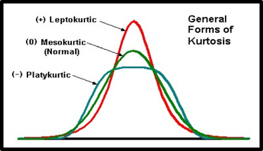
Another characteristic of a frequency distribution is Kurtosis.
--Kurtosis refers to the flatness or the peakedness of a distribution.
—A distribution can be Leptokurtic, Mesokurtic or Platykurtic.
Leptokurtic Distribution
A distribution with a high peak. It is more peaked than the normal distribution.
Mesokurtic Distribution
A distribution with a medium peak and resembles a bell shape. It is also called a normal curve.
Platykurtic Distribution
A distribution with low peak. It is flatter than the normal curve.
Measure of Central Tendency
We can gain useful information from raw data by organizing them into a frequency distribution and then presenting the data by using various graphs. However, we might be interested in knowing more about our data and describing the data in greater depth. This can be done through the Measure of Central Tendency ( MCT).
There are Three types of Measures of Central Tendency:
There are Three types of Measures of Central Tendency:
- Mean: The average value of the data set
- Median: The middle value in a data set
- Mode: The most frequent value in a data set
—The Use of MCT depends on the scale of measurement of the data:
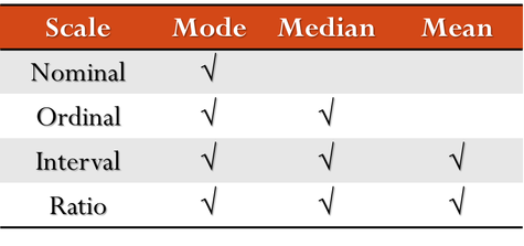
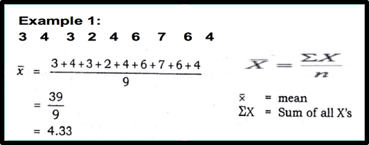
Mean
- Mean is the most frequently used MCT. It is the average value in a data set.
- Mean can be calculated for quantitative data ( Interval & Ratio data).
- Mean cannot be calculated for qualitative data ( nominal & ordinal data).
- It is very much susceptible to the presence of extreme values ( high or low values called outliers). In other words, if a data set has an outlier, the value of mean will not be valid. So, data set should be checked for error before performing any analysis. (Cases with values well above or well below the majority of other cases are called outliers)
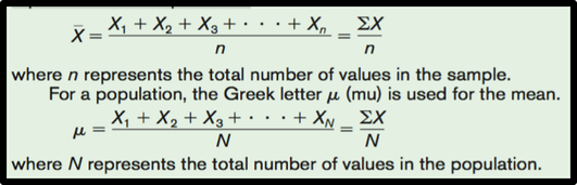
- The mean is the sum of the values, divided by the total number of values.
- The symbol x̄ (X Bar) represents the sample mean.
- The symbol μ represents the population mean.
Median
- It is also called 50th percentile.
- Median is the middle value in a data set.
- Median is not sensitive to extreme values. The median is affected less than the mean by extremely high or extremely low values.
- It is used to find out whether a data value falls into the upper half or lower half of the distribution. For example, if we found that the median income for college professors is $40,000, it means that one-half of the professors earn more than $40,000 and one-half earn less than $40,000.
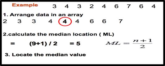
- For finding median of a data set, first, we should arrange data in order (Arrange from lowest to highest values). Second, we should calculate the median location [( n+1)/2] and finally locate the median value.
- The symbol for the median is MD.
- 1, 2, 3, 6 ,8, 10,14 MD=6
- When there are an odd number of values in the data set, the median will be an actual data value.
- When there are an even number of values in the data set, the median will fall between two given values.
Mode
- Mode corresponds to value with the highest frequency.
- Mode can be calculated for nominal data such as religious preference, gender, or political affiliation.
- Mode is not sensetive to extreme values ( outliers)
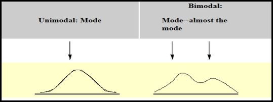
- A data set can be Unimodal, Bimodal, or Multimodal.
- A unimodal data set has only one value with the greatest frequency
- A bimodal data set has two values with the same greatest frequency (both values are considered to be the mode )
- A multimodal data set has more than two values with the same greater frequency (each value is used as the mode)
- For example: 6 , 6, 6, 7, 7, 9, 9, 9, 10, 10,10
- When no data value occurs more than once, the data set is said to have no mode.
Relationship of the Mean, Median and Mode
--If a frequency distribution has a symmetrical frequency curve, the mean, median, and mode are equal.
- If a frequency distribution is positively skewed , then mean is grater than median and median is grater than mode.
- If a frequency distribution is negatively skewed, then mean is less than median and median is less than mode.
| |
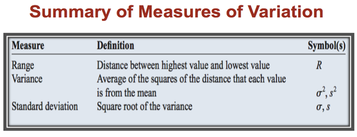
Measures of Distribution
Although measure of central tendency provides us with information on Mean, Media, and Mode, additional information about the data can be supplemented by measures of Dispersion. The main purpose of measures of dispersion is to get as much as possible a true picture of the data. Dispersion indicates the spread or variability of the data in a distribution. In other words, dispersion is the amount of spread of data about the centre of the distribution.
Measures of distribution include:
- Range
- Variance
- Standard deviation
Two data set can have similar means but may have differences in dispersion.
For example: Data set A & B
For example: Data set A & B
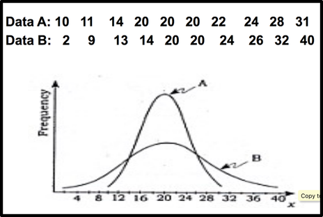
| The above data sets ( A& B) have similar mean but have different dispersion. Data set B is more dispersed or spread from its mean. Data set A is more clustered about the mean ( majority of data cluster around the mean ). Range |
Range is the simplest measure of dispersion. Determination of range is based on only two values in a data set ( highest value and lowest value) and is easy to be computed.
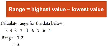
A large range indicates a more dispersed data set about the mean while a small range exhibits a more clustered data about its mean.
Range is very sensitive to outlier. In its calculation, range ignores all values in the data set except the two values( highest and lowest values). In the case that the highest and lowest values are unsusually extremes, value of range will not be valid.
Range is very sensitive to outlier. In its calculation, range ignores all values in the data set except the two values( highest and lowest values). In the case that the highest and lowest values are unsusually extremes, value of range will not be valid.
Variance
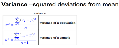
Variance is a statistical measure that quantifies the amount of variability or dispersion in a dataset. It measures how much the individual observations in a dataset deviate from the Mean of the dataset. If the values are near the mean, the variance will be small. In contrast, if the values are far from the mean, the variance will be large. Therefore, the higher variance indicates the greater variability, and the smaller variance indicates the lower variability.
Mathematically, variance is the average of the squared differences of each observation from the mean of the dataset. In other words, it is the average of the squared deviations of each data point from the mean. The above formula can be used to calculate variance.
Please watch the following video to learn more about variance:
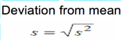
Standard Deviation
- Standard deviation is the most important and frequently used measure of dispersion.
- Standard deviation which is denoted by S is the positive square root of the variance; and vice versa, squaring the standard deviation gives the variance.
- Standard deviation indicates how far the individual responses to a question vary or deviate from the mean.
- Standard deviation tells the researcher how spread out the responses are, are they concentrated around the mean or scattered far and wide.
- The variance and standard deviation of a data set can never be negative.
Using Excel to Calculate Measures of Dispersion
| 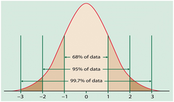 |
- A normal distribution can be used to describe a variety of quantitative variables.
- A normal distribution curve is bell-shaped.
- The mean, median, and mode are equal and are located at the center of the distribution.
- A normal distribution curve is unimodal ( it has only one mode).
- The curve is symmetric about the mean. It means that the right portion of the distribution is equal to the left portion of the distribution.
- The curve is continuous; that is, there are no gaps or holes.
- The curve never touches the x axis. Theoretically, no matter how far in either direction the curve extends, it never meets the x axis—but it gets increasingly closer.
- The total area under a normal distribution curve is equal to 1.00, or 100%.
- In the normal distribution, about 68% of the data fall within 1 standard deviation of the mean ; about 95% of the data fall within 2 standard deviation of the mean; and about 99.7% of data fall within 3 standard deviation of the mean.
Normal curves have different shapes and can be used to represent different variables.
The shape and position of a normal distribution curve depend on two parameters, the mean and the standard deviation. Each normally distributed variable has its own normal distribution curve, which depends on the values of the variable’s mean and standard deviation.
The shape and position of a normal distribution curve depend on two parameters, the mean and the standard deviation. Each normally distributed variable has its own normal distribution curve, which depends on the values of the variable’s mean and standard deviation.
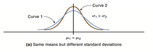
The above figure shows two normal distributions with the same mean values but different standard deviations. The larger the standard deviation, the more dispersed, or spread out, the distribution is.
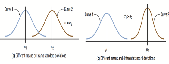
Figure (b) shows two normal distributions with the same standard deviation but with different means. These curves have the same shapes but are located at different positions on the x axis. Figure(c) shows two normal distributions with different means and different standard deviations.
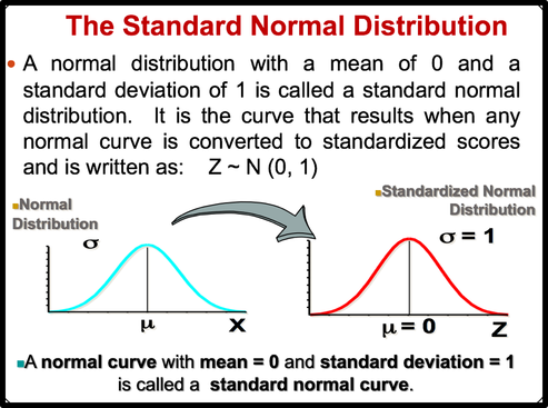
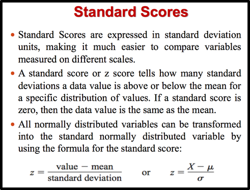
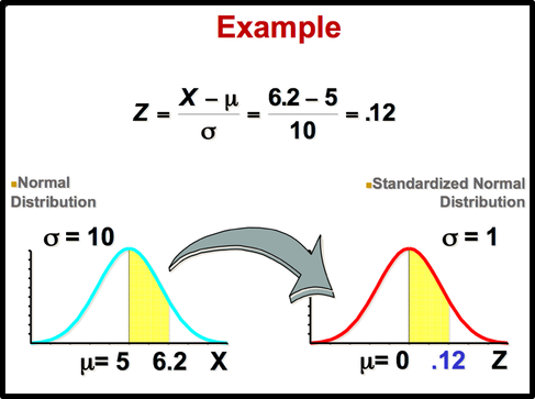
All normally distributed variables can be transformed into the standard normally distributed variable by using Standard Score (Z).
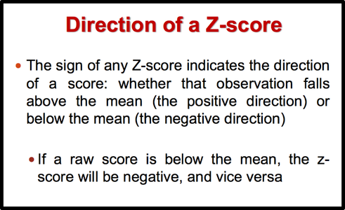
Standard Score indicates the relative location of the observation in a data set. In other words, it indicates how many standard deviation a data value is above or below the mean.
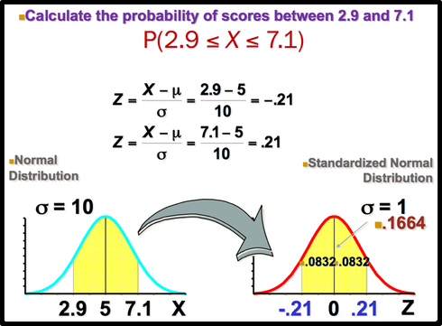
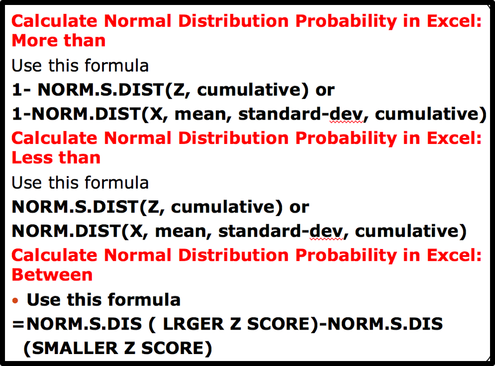
Normal Distribution Probability
Sometimes we want to know not only the relative location of observation in a data set but also the probability occurence of observation in a data set. In this case, we should calcuate the the area under the curve which is called Probability.
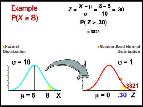
You can use z table to find the probability .
Z value can be calculated by using NORM.S.INV(probability) function. For example, Z value to the left of the mean for the 98.87% of the area under the distrubution curve will be -2.28.
If we want to find the observation value, we can use the NORM.INV (probability, mean, standard deviation) Function.
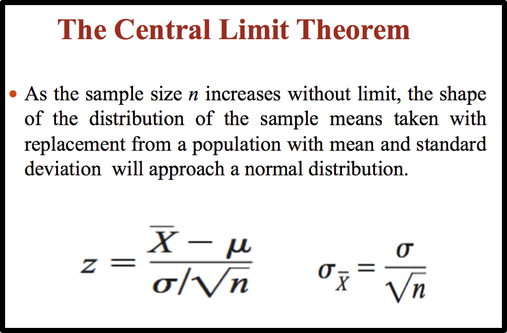
The Central Limit Theorem is the cornerstone of statistics. It is an important concept that should be considered when performing any type of data analysis. Suppose that we are interested in estimating average hight among young people in Vancouver. Collecting data from all young people in Vancouver is impractical. If we want to collect data from all young people, we should spend a lot of time, money, energy. So, we should select the sample from the population.
We should keep in mind, However, the sample should be representative of the population to ensure that we can generalise the findings from the research sample to the population as a whole. Hence, appropriate sample size should be selected for our study.
Based on the Central Limit Theorem, as the sample size increases, it approaches the size of the entire population. It also approaches all the charecteristics of the population. Therefore sampling error will decrease.
The mean of the sample mean will get the same as the population mean. The standard deviation of the sample mean will get smaller than the standard deviation of the population and it will be calculated by dividing the population standard deviation by the square root of the sample size. .
Based on the Central Limit Theorem:
1. The mean of the sample means = mean of the population
2. If the population is normal then sample means will have a normal distribution.
3. If the population is not normal but sample size is greater than 30 then sampling distribution of sample means approximates a normal distribution.
Drawing Normal distribution Density Curve with Excel
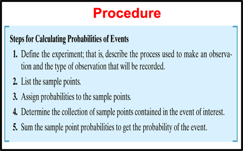
Determine Sample Spaces and Find the Probability of an Event
Probability is a concept that is widely used in everyday life. To a certain extent the term can be synonymous to likelihood of an event to happen. In other words, Probability can be defined as the chance of an event occurring. Many people are familiar with probability from observing or playing games of chance, such as card games, slot machines, or lotteries. In addition to being used in games of chance, probability theory is used in the fields of insurance, investments, and weather forecasting and in various other areas. For example, a stock broker can use probability to determine the rate of return on a client's investments. Finally, probability is the basis of inferential statistics. For example, predictions are based on probability, and hypotheses are tested by using probability.
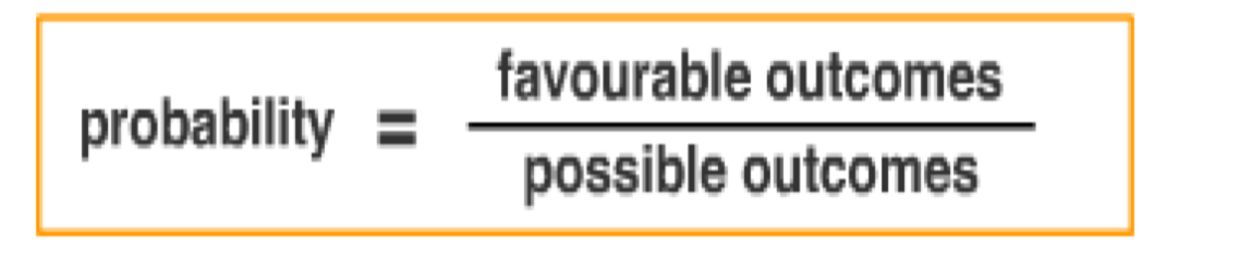
The oldest and most commonly used definition of probability is :
—If an event can occur in A ways and can fail to occur in B ways, and if all possible ways are equally likely , then the probability of its occurrence is A/ ( A+B), and the probability of its failing to occur is B/ ( A+B).
The oldest and most commonly used definition of probability is :
—If an event can occur in A ways and can fail to occur in B ways, and if all possible ways are equally likely , then the probability of its occurrence is A/ ( A+B), and the probability of its failing to occur is B/ ( A+B).
we should be familiar with basic terminology and rules in probability in order to better understand the application of probability . They are as follows:
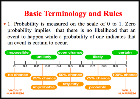
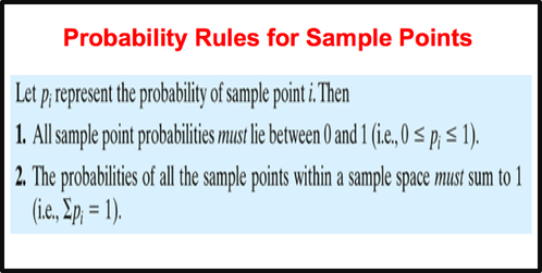
Probability is measured on the scale of 0 to 1. Zero probability indicates that there is no chance that an event will happen while a probability of one indicates that an event is certain to occur.
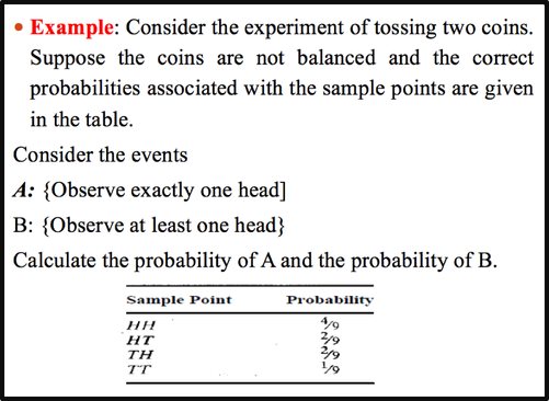
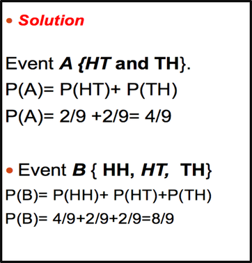
When we toss a coin, there is a chance that two things happen, tail or head, both have equal chance to happen. A chance to obtain a head is 50% and a chance to obtain a tail is also 50%.
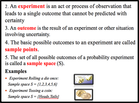
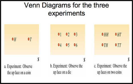
Suppose a coin is tossed once and the up face is recorded. The result we see and record is called an observation or outcome and the process of making an observation is called an experiment.
The set of all possible outcomes of a probability experiment is called a sample space, which is usually denoted by S.
The basic possible outcomes to an experiment are called sample points . In other words, sample points are elements of sample space.
The total probability of all sample points within a sample space is equal 1.
When we toss a coin, there is a chance that two things happen, tail or head, both have equal chance to happen. A chance to obtain a head is 50% and a chance to obtain a tail is also 50%.
Suppose a coin is tossed once and the up face is recorded. The result we see and record is called an observation or outcome and the process of making an observation is called an experiment.
The set of all possible outcomes of a probability experiment is called a sample space, which is usually denoted by S.
The basic possible outcomes to an experiment are called sample points . In other words, sample points are elements of sample space.
The total probability of all sample points within a sample space is equal 1.
Some sample spaces for various probability experiments are shown here.
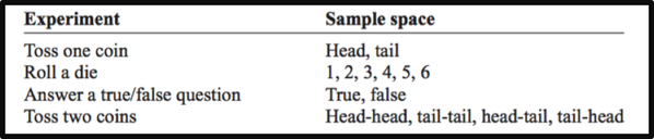
Just as graphs are useful in describing sets of data, a pictorial method for presenting the sample space will often be useful.
we can use Venn diagrams or tree diagrams to present sample space.
A tree diagram is a device consisting of line segments emanating from a starting point and also from the outcome point. It is used to determine all possible outcomes of a probability experiment.
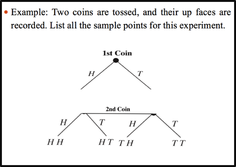
Example
—A retail computer store sells two basic types of personal computers (PCs): standard desktop units and laptop units. Thus the owner must decide how many of each type of PC to stock. An important factor affecting the solution is the proportion of customers who purchase each type of PC. Show how this problem might be formulated in the framework of an experiment with sample points and a sample space. Indicate how probabilities might be assigned to the sample points. (The store's records indicates that 80% of its customers purchase desktop units).
Solution
--D: {The customer purchases a standard desktop unit}
—L: (The customer purchases a laptop unit)
—It might be reasonable to approximate the probability of the sample point D as .8 and that of the sample point L as .2.
Here we see that sample points are not always equally likely. So assigning probabilities to them can be complicated, particularly for experiments that represent real applications (as opposed to coin and die-toss experiments).
What is an event?
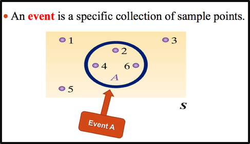
An event is the subset of sample space.
An event can be one outcome or more than one outcome. For example, if a die is rolled and a 6 shows, this result is called an outcome, since it is a result of a single trial. An event with one outcome is called a simple event. The event of getting an odd number when a die is rolled is called a compound event, since it consists of three outcomes or three simple events. In general, a compound event consists of two or more outcomes or simple events.
There are three basic interpretations of probability:
Classical probability assumes that all outcomes in the sample space are equally likely to occur. For example, when a single die is rolled, each outcome has the same probability of occurring. Since there are six outcomes, each outcome has a probability of 1/ 6. When a card is selected from an ordinary deck of 52 cards, you assume that the deck has been shuffled, and each card has the same probability of being selected. In this case, it is 1/52 .
Relative Frequency probability is the ratio of the occurrence of a singular event and the total number of outcomes. This is a tool that is often used after you collect data. You can compare a single part of the data to the total amount of data collected.
Subjective probability is a type of probability derived from an individual's personal judgment about whether a specific outcome is likely to occur. It is not based on mathematical calculations . It reflects the subject's opinions and past experience. Subjective probabilities differ from person to person, and contains a high degree of personal bias.
The Probability of an Event
An event can be one outcome or more than one outcome. For example, if a die is rolled and a 6 shows, this result is called an outcome, since it is a result of a single trial. An event with one outcome is called a simple event. The event of getting an odd number when a die is rolled is called a compound event, since it consists of three outcomes or three simple events. In general, a compound event consists of two or more outcomes or simple events.
There are three basic interpretations of probability:
- Classical probability
- Empirical or relative frequency probability
- Subjective probability
Classical probability assumes that all outcomes in the sample space are equally likely to occur. For example, when a single die is rolled, each outcome has the same probability of occurring. Since there are six outcomes, each outcome has a probability of 1/ 6. When a card is selected from an ordinary deck of 52 cards, you assume that the deck has been shuffled, and each card has the same probability of being selected. In this case, it is 1/52 .
Relative Frequency probability is the ratio of the occurrence of a singular event and the total number of outcomes. This is a tool that is often used after you collect data. You can compare a single part of the data to the total amount of data collected.
Subjective probability is a type of probability derived from an individual's personal judgment about whether a specific outcome is likely to occur. It is not based on mathematical calculations . It reflects the subject's opinions and past experience. Subjective probabilities differ from person to person, and contains a high degree of personal bias.
The Probability of an Event
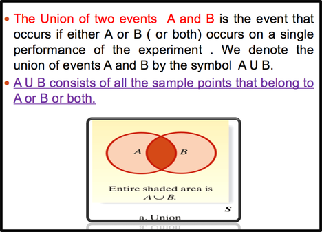
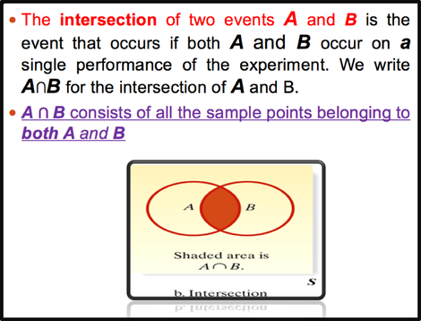
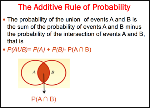
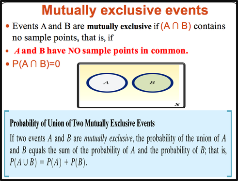
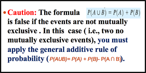
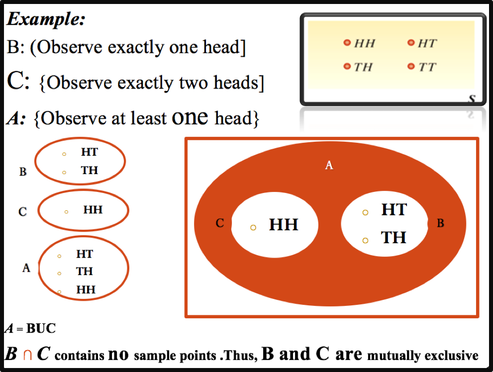
Unions and Intersections
Solution
Example
—Hospital records show that 12% of all patients are admitted for surgical treatment, 16% are admitted for obstetrics, and 2% receive both obstetrics and surgical treatment. If a new patient is admitted to the hospital, what is the probability that the patient will be admitted either for surgery, obstetrics, or both? Use the additive rule of probability to arrive at the answer.
—Solution
A: {A patient admitted to the hospital receives surgical treatment]
—B: {A patient admitted to the hospital receives obstetrics treatment)
—P(A)=.12
—P(B)=.16
—P(A ∩ B)=.02
—P(AUB)= P(A) + P(B)- P(A ∩ B)
— =.12+.16-.02=.26
—26% of all patients admitted to the hospital receive either surgical treatment, obstetrics treatment, or both.
--
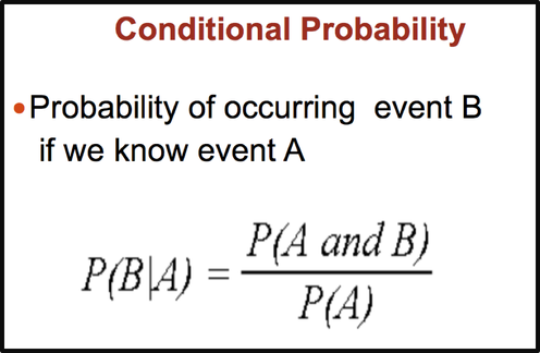
All probabilities that we dicussed were unconditional probabilities because no special conditions are assumed. Sometimes, we have additional knowledge of an experiment that might affect the outcome of an experiemtn. A probability that reflects such additional knowledge is called the conditional probability of the event.
 |
 RSS Feed
