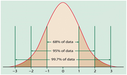
Normal curves have different shapes and can be used to represent different variables. The shape and position of a normal distribution curve depend on two parameters, the mean and the standard deviation. Each normally distributed variable has its own normal distribution curve, which depends on the values of the variable’s mean and standard deviation. 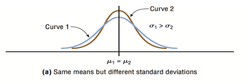 The above figure shows two normal distributions with the same mean values but different standard deviations. The larger the standard deviation, the more dispersed, or spread out, the distribution is. 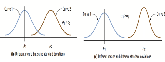 Figure (b) shows two normal distributions with the same standard deviation but with different means. These curves have the same shapes but are located at different positions on the x axis. Figure(c) shows two normal distributions with different means and different standard deviations. All normally distributed variables can be transformed into the standard normally distributed variable by using Standard Score (Z). Standard Score indicates the relative location of the observation in a data set. In other words, it indicates how many standard deviation a data value is above or below the mean. 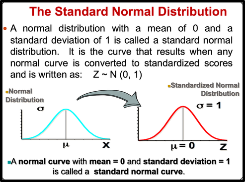 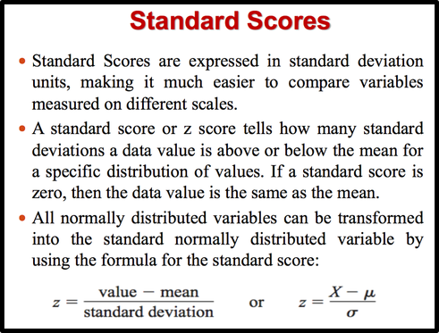   Normal Distribution ProbabilitySometimes we want to know not only the relative location of observation in a data set but also the probability occurence of observation in a data set. In this case, we should calcuate the the area under the curve which is called Probability.  You can use z table to find the probability .  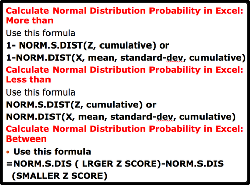 Z value can be calculated by using NORM.S.INV(probability) function. For example, Z value to the left of the mean for the 98.87% of the area under the distrubution curve will be -2.28. If we want to find the observation value, we can use the NORM.INV (probability, mean, standard deviation) Function. 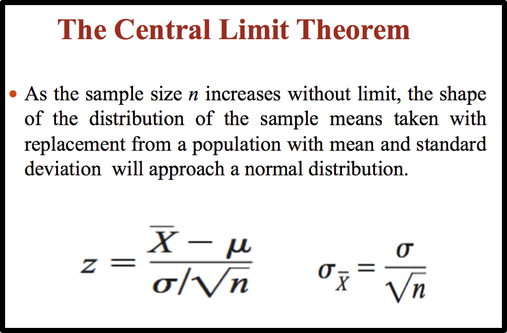 The Central Limit Theorem is the cornerstone of statistics. It is an important concept that should be considered when performing any type of data analysis. Suppose that we are interested in estimating average hight among young people in Vancouver. Collecting data from all young people in Vancouver is impractical. If we want to collect data from all young people, we should spend a lot of time, money, energy. So, we should select the sample from the population. We should keep in mind, However, the sample should be representative of the population to ensure that we can generalise the findings from the research sample to the population as a whole. Hence, appropriate sample size should be selected for our study. Based on the Central Limit Theorem, as the sample size increases, it approaches the size of the entire population. It also approaches all the charecteristics of the population. Therefore sampling error will decrease. The mean of the sample mean will get the same as the population mean. The standard deviation of the sample mean will get smaller than the standard deviation of the population and it will be calculated by dividing the population standard deviation by the square root of the sample size. . Based on the Central Limit Theorem: 1. The mean of the sample means = mean of the population 2. If the population is normal then sample means will have a normal distribution. 3. If the population is not normal but sample size is greater than 30 then sampling distribution of sample means approximates a normal distribution. Drawing Normal distribution Density Curve with Excel
0 Comments
|
 RSS Feed
