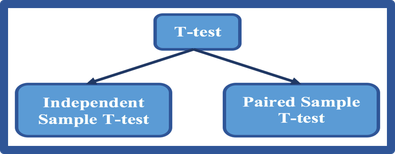
 z test is used to test the difference between two means when the population standard deviations are known and the variables are normally or approximately normally distributed. In many situations, however, these conditions cannot be met—that is, the population standard deviations are not known. In these cases, a t test is used to test the difference between means. There are a number of different types of t-tests. The two that will be discussed here are: • Independent-samples t-test, used when we want to compare the mean scores of two different groups of people or conditions; and • Paired-samples t-test, used when we want to compare the mean scores for the same group of people on two different occasions, or when we have matched pairs. In both cases, we are comparing the values on some continuous variable for two groups or on two occasions. If we have more than two groups or conditions, we will need to use analysis of variance instead. AssumptionsFor both of the t-tests that I discuss here, there are a number of assumptions that we will need to check before conducting these analyses. Level of measurement Each of the parametric approaches assumes that the dependent variable is measured at the interval or ratio level; that is, using a continuous scale rather than discrete categories. When we want to design our study, we should try to make use of continuous, rather than categorical for the dependent variable. This gives us a wider range of possible techniques to use when analyzing our data. Random sampling Data should be collected using a random sample from the population. Independence of observations The observations that make up our data must be independent of one another; that is, each observation must not be influenced by any other observation. Violation of this assumption, according to Stevens (1996, p. 238), is very serious. There are a number of research situations that may violate this assumption of independence. For example:
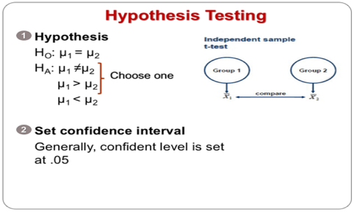
Normal distribution For parametric techniques, it is assumed that the populations from which the samples are taken are normally distributed. In a lot of research scores on the dependent variable are not normally distributed. Fortunately, most of the techniques are reasonably 'robust' or tolerant of violations of this assumption. With large enough sample sizes (e.g. 30+), the violation of this assumption should not cause any major problems. Normality of our variables can be checked using histograms, stem and leaf display, Box plot. WE can also check the value of Skewness and mean, median, and mode of our variable (Mean=Median=mode). Homogeneity of variance Samples that are obtained from populations should have equal variances. This means that the variability of scores for each of the groups is similar. Independent Sample T-test 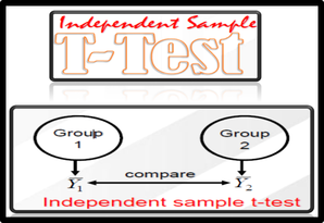 Purpose of Independent sample t-test—To compare differences between two (2) independent group means Requirements ►DV–Interval or ratio ►IV–Nominal or ordinal (k=2)
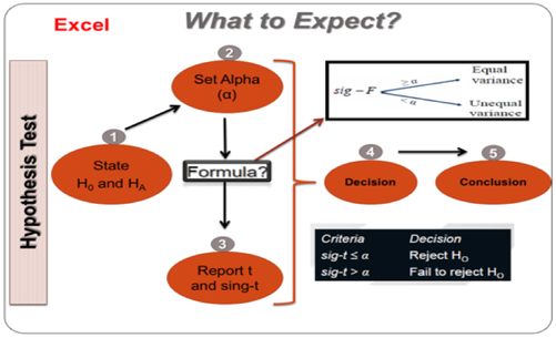
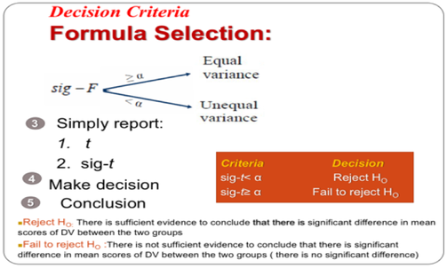
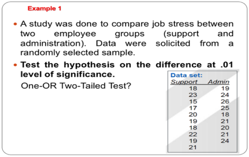 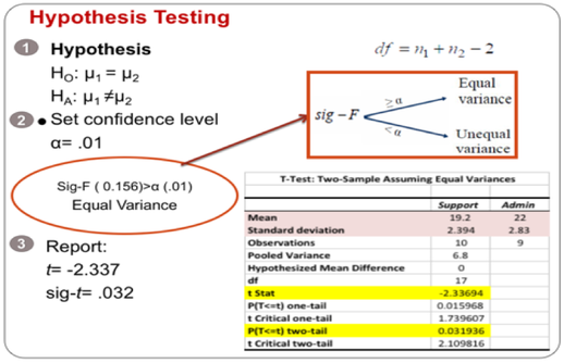 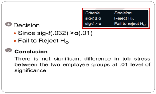 Interpretation of output from independent-samples t-test Step 1: Checking the information about the groups Excel gives us the mean and standard deviation for each of our groups (in this case, Support/ Admin). It also gives us the number of people in each group (N). We should always check these values first. Are the N values for support and Admin correct? Or are there a lot of missing data? If so, we should find out why. Perhaps we have entered the wrong code for Support and females (0 and 1, rather than 1 and 2). We should check our codebook. Step 2: Checking assumptions The independent sample t-test assumes the variances of the two groups we are measuring are equal in the population. If our variances are unequal, this can affect the Type I error rate. We should run the F-test two sample for variances in Excel to check the equality of variances. This tests whether the variance (variation) of scores for the two groups (Support and Admin) is the same. If Sig-F is grater than the significance value (Sig-F ≥ œ), the T-test: two sample assuming equal variances can be used. If Sig-F is less than the level of significance (Sig-F≤ œ), the test for equality of variances is statistically significant. It indicates that the group variances are unequal in the population. We can correct this violation by using the T-test: two sample assuming unequal variances. In this case, Sig-F is larger than alpha value so we can use the T-test: two sample assuming equal variances. We should also check other assumptions such as level of measurement, random sampling, independence of observations, and normality of our data. Step 3: Assessing differences between the groups To find out whether there is a significant difference between our two groups, we should compare P-value ( Sign-t) with the level of significance.
In the example presented in the output above, the P value (Sig. t- 2-tailed) is .03. As this value is above the required cut-off of .01, we conclude that there is not a statistically significant difference in the mean Job stress scores for Support and Admin group. Calculating the effect size for independent-samples t-test One way that we can assess the importance of our finding is to calculate the effect size. Effect size statistics provide an indication of the magnitude of the differences between our groups (not just whether the difference could have occurred by chance). There are a number of different effect size statistics, the most commonly used are eta squared and Cohen’s d. Eta squared can range from 0 to 1 and represents the proportion of variance in the dependent variable that is explained by the independent (group) variable. We can use a formula to calculate the eta squared. 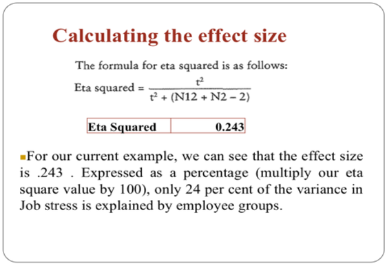 Presenting the results for independent-samples t-test The results of the analysis can be presented as follows: An independent-samples t-test was conducted to compare the job stress scores for Support and Admin groups. There was no significant difference in the mean Job stress scores for Support (M = 19.2, SD = 2.39) and Admin groups (M = 22, SD = 2.83) at 0.01 (t = -2.336, p = .03, two-tailed). Eta squared was 0.243 ( 24% of of variance in the Job stress is explained by the employee groups). The magnitude of the differences in the means (mean difference = 2.8,) was 1.07 .
1 Comment
Hey there, just wanted to drop by and say that I found your article on Independent Sample T-test really informative and well-written! I appreciate the clear explanation of the assumptions that need to be checked before conducting the analysis and the step-by-step guide on how to interpret the output. It's great to have a resource that breaks down the technical jargon into easily understandable language. Keep up the good work! Leave a Reply. |
Categories
All
|
 RSS Feed
